Warming oceans weaken sea and land winds in coastal cities – Nature Climate Change

Forcing SST

Traditional low-resolution sea surface temperature datasets cannot resolve local warming disparities in coastal areas, whereas kilometer-scale resolution data depict land-sea temperature gradients 4). Comparing with observations, we find that SST from BCC-CSM2-MR shows strong consistency with both reanalysis datasets and satellite assimilation data in capturing monthly variations in SST among several CMIP6 GCMs (ACCESS-ESM1.5, BCC-CSM2-MR, CanESM5, CESM2, and EC-Earth3) (Supplementary Fig. 5). Moreover, statistical analysis confirms that the BCC-CSM2-MR results show high reliability across several indicators (Supplementary Text 5).

This study advances ocean surface temperature parameterization in a WRF model through the following technical workflow: Land and ocean mask data were extracted from the meteorological input file (met_em) using the MODIS land use classification system with water bodies corresponding to category 16. The boundaries of the oceanic grid were precisely identified by geographic coordinate transformation (WRF Lambert projection to the WGS84 coordinate system). A set of high-resolution SST data from CMIP6 was spatially and temporally aligned with the WRF ocean domain using a spatiotemporal matching algorithm (Supplementary Figure 6). The daily SST fields were dynamically integrated into the WRF initial conditions and replaced the static SST parameters. Future daily and diurnal sea surface temperatures based on SSP 245 and SSP 585 scenarios were applied to examine the impact of future ocean warming on SLB days in the same way as introduced above for the historical case. With advances in remote sensing and multi-source data assimilation techniques, ultra-high-resolution SST products (e.g., GHRSST) provide opportunities for cross-validation using multiple datasets. Our comparison shows that the reanalysis data shows the highest correlation with the BCC simulations, followed by the GHRSST satellite observations.⁴² (Supplementary Text 5). SLB daily-scale residual biases can arise from uncertainties in the near-shore sea surface temperature field and nearshore wind representation, especially for cities with complex coastlines.

Model configuration

The WRF model is a mesoscale weather model and assimilation system. It has been widely adopted in most countries around the world as a tool for both operational and research applications in mesoscale weather forecasting. The WRF model used in this study is v.4.2.2, which includes specific physical process parameterization settings (Supplementary Text 6).

In this study, we conducted an SST-focused sensitivity analysis using enhanced high-resolution SST modeling results combined with the WRF model using a controlled variable experimental design. The simulations, conducted under a controlled parameterization with fixed land use, anthropogenic heat, and surface roughness, employed the same meteorological field as initial and boundary conditions. A comparative analysis of changes in the number of SLB days under different sea surface temperature conditions quantitatively revealed the impact of anomalous sea surface temperature increases on SLB patterns.

The simulation period runs from January 1st to December 31st, for a total of 365 days each year. Under the guidance of some initial experiments, a 22-day model spin-up was implemented to optimize computational efficiency and minimize initial field interferences. Two nested domains were used with spatial resolutions of 27 km and 9 km (Supplementary Text 7). Sea surface temperature data (SSP245 and SSP585) for 1970, 2010, and 2050 simulated by the BCC-CSM2-MR model were used for forcing measurements at 6-h intervals.

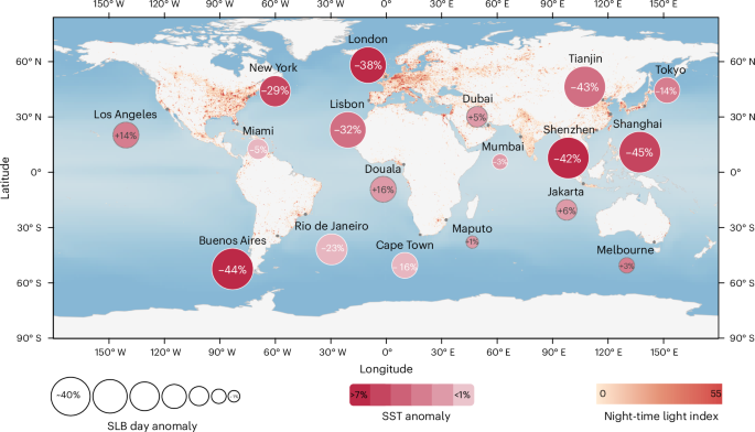
Prior research was considered in selecting the points of interest for this study.⁴³ This includes factors such as the size of the city, its latitude and longitude distribution, the continent on which the city is located, and the climate zone that the city represents. Our goal was to achieve comprehensive coverage to discuss the potential impact of SST changes on SLB from several perspectives (Supplementary Text 6 and Supplementary Table 1). To select the study area, this study first identified the global climate zones that are primarily affected by SLB. Nighttime light data helped select the metropolises with the highest light intensity index within these climate zones (Figure 1)^41,44. The final spot selection integrated several criteria, including city size, outstanding wind patterns, proximity to the coast, and climate characteristics. The city-coast boundary is drawn using land-use data, with two nested domains organized around the urban land area adjacent to the coastline. The internal domain is designed to maintain approximately equal representation of land and ocean (approximately 50% each) and ensure balanced atmospheric interactions. This balanced configuration minimizes the effects of unbalanced boundary conditions from a single peripheral direction and reduces potential biases introduced by human intervention in the experimental design.

data collection

High-resolution SST data from CMIP6 (BCC-CSM2-MR model, 0.3° to 1° spatial resolution from equator to poles)⁴⁵ used in this study. BCC’s historical sea surface temperature simulation data spans from 1950 to 2014. In this study, we also selected the data for 2050 under two emission scenarios: SSP 245 and SSP 585 to analyze the changes in SLB under different future emission scenarios. In this study, we use four other high-resolution SST datasets from CMIP6, namely ACCESS-ESM1.5 (~1.25° × 1.875°), CanESM5 (~2.8° × 2.8°), CESM2 (~1.25° × 0.9°), and EC-Earth3 (~1.0° × 1.0°) to We evaluated the impact of between-model differences in Simulation results. For meteorological data, this study used the Final Operational Global Analysis (FNL) dataset provided by the National Center for Environmental Prediction.⁴⁶. The FNL dataset produced by the Global Data Assimilation System contains various meteorological parameters with a spatial resolution of 0.25° × 0.25° and is updated every 6 hours. FNL data are widely used in meteorological research and numerical weather prediction models, and are a common data source for numerical simulations. All other parameters and input data were kept at the default model settings to control the influence of other variables on the simulation. The land use classification follows the MODIS land use classification standard and the simulation is based on the land use parameters provided in WRF v.4.2.2.

Criteria for identifying SLB days

According to the basic definition, an SLB day must meet the criteria that both sea and land breezes occur during the day and that an obvious transformation process is observed.²⁹. Additionally, this study can only identify as SLB days those days that meet all of the following criteria, including temperature difference, specific wind direction, wind speed limit, and sustained intensity. A sea breeze was defined as a case where the wind direction corresponds to the sea breeze area and the temperature at the ocean observatory is lower than that at the observatory in the urban area. Similarly, land breeze was defined as when the wind direction was compatible with the land wind regime and the temperature at ocean stations was higher than at urban stations (Supplementary Table 1). Although the above two conditions satisfy the basic definition of an SLB day, this method does not use a specific time for determining sea breeze or land breeze, as described in previous studies. This method excluded cases where the observed wind speed exceeded 10 ms.⁻¹ They are installed at coastal observation stations to prevent disruption from large weather systems. This method took into account the time and intensity of SLB to identify SLB days. A typical SLB day requires both sea and land breezes to occur over 4 hectares. In addition, the wind speed of the sea breeze must be 1m・s or more.^-1 The wind speed of land wind should be 0.5ms or more.^-1. All these criteria have a logical relationship. Temperature difference is the essential cause and basic criterion of SLB. Wind direction criteria include wind direction and wind speed, and are specialized depending on the shape of the coastline and the distribution of land and sea. Sustained strength is then considered to ensure that SLB is evident.

Unsupervised cluster analysis

This study focuses on unsupervised machine learning (k-means clustering) to depict the relationship between SST variability and the frequency of sea breeze days and identify three distinct coastal response clusters. Clustering analysis was achieved by constructing a two-dimensional feature vector from the daily frequency of sea surface temperature anomalies and sea breezes to geometrically characterize the data. Iteratively calculates the Euclidean distance between data points and cluster centroids and assigns samples to clusters based on a minimum distance threshold. To determine the optimal number of clusters (k) Since there was no prior knowledge about the class categories, the sum of error squares evaluation method was applied. After several repetitions, k = 3 was identified as the optimal classification number that balances computational efficiency and cluster stability. The specific mathematical model used is:

objective function JDefined by Equation (1), we quantify the total variance within a cluster as the sum of the squared Euclidean distances between each data point. ×_j and its corresponding cluster centroid meter_{I .} kis the number of clusters, C_I means IThe th cluster containing all assigned data points. The data points in the feature space are: ×_j and meter_I center of gravity (average position) IIteratively computed th cluster.

In equation (2), |C_I|Indicates the cardinality (number of data points) in the cluster C_I. This metric reflects the statistical weight of cluster centroids. meter_Iquantifies the ability to represent the spatial distribution of elements. C_I During each iteration, all data points are assigned by Equation (3). ×_j to the nearest cluster centroid C_I.

Furthermore, we used the Monte Carlo resampling method to validate the clustering results. The average silhouette coefficient across all iterations was 0.82, confirming the overall validity and stability of the identified clusters (Supplementary Text 8).

Spatiotemporal statistical downscaling method

How to generate dynamically consistent atmospheric and boundary conditions from CMIP6 output. This approach allows each future scenario to evolve under corresponding large-scale atmospheric conditions, rather than assuming a static IC/BC field. Specifically, we established variable mapping between the CMIP6 dataset and WRF input files (Supplementary Text 4 and Supplementary Table 3). Based on the time stamps in the WRF files, we used a nearest-neighbor time matching algorithm to align the CMIP6 time slices, followed by bilinear spatial interpolation to transform the CMIP6 data from the native grid to the WRF domain. Special longitude adjustments were applied to ensure continuity across the International Date Line (0° to 360° and -180° to 180° systems). For vertical interpolation, we performed logarithmic pressure remapping of the pressure level variable to maintain monotonicity and ensure physical consistency between layers. Comprehensive dimension checking, alignment verification, and post-interpolation verification were also implemented to ensure the physical validity of the downscaled fields.